Violation Frequency

knitr::opts_chunk$set(
  warning = FALSE,
  message = FALSE)

library(tidyverse)
library(dplyr)
library(rvest)
library(purrr)
library(ggplot2)
library(modelr)
library(mgcv)
library(patchwork)
library(viridis)
library(fastDummies)
set.seed(1)

childcare_inspection_df = read_csv("./data/DOHMH_Childcare_Center_Inspections.csv") %>% 
janitor::clean_names() %>% 
distinct() %>% 
    select(center_name, borough, zip_code, status, age_range, maximum_capacity,program_type, facility_type, 
         child_care_type, violation_category,
         violation_status,violation_rate_percent:average_critical_violation_rate,regulation_summary,
         inspection_summary_result) %>%
  drop_na(zip_code, age_range, violation_rate_percent,public_health_hazard_violation_rate, critical_violation_rate) %>% 
  filter(maximum_capacity != 0) %>% 
  mutate(
    educational_worker_ratio = total_educational_workers/maximum_capacity,
    program_type = tolower(program_type),
    facility_type = tolower(facility_type),
    borough =  as.factor(borough),
    status = as.factor(status),
    program_type = as.factor(program_type),
    facility_type = as.factor(facility_type),
    child_care_type = as.factor(child_care_type),
    age_range = as.factor(age_range)
  ) %>% 
  filter(program_type != "school age camp")

center_specific_df = childcare_inspection_df %>% 
  relocate(center_name, program_type) %>% 
  group_by(center_name, program_type) %>% 
  mutate(
    n_na = sum(is.na(violation_category)), 
    n_violation = sum(!is.na(violation_category)), 
    rate = n_violation/(n_violation + n_na)) %>% 
  arrange(center_name, program_type)

Number of violations by program type

Histogram plot

frequency_program_type = childcare_inspection_df %>% 
  count(program_type) %>% 
  mutate(
    program_type = fct_reorder(program_type, n)
    ) %>% 
  ggplot(aes(x = program_type, y = n, fill = program_type)) + 
  geom_bar(stat = "identity") + 
  labs(
    title = "Frequency of Violations by Program Type",
    x = "Program Type",
    y = "Number of Violations",
    fill = "program_type") +
  theme(axis.text.x = element_text(angle = 0, hjust = 0.5),plot.title = element_text(hjust = 0.5))
frequency_program_type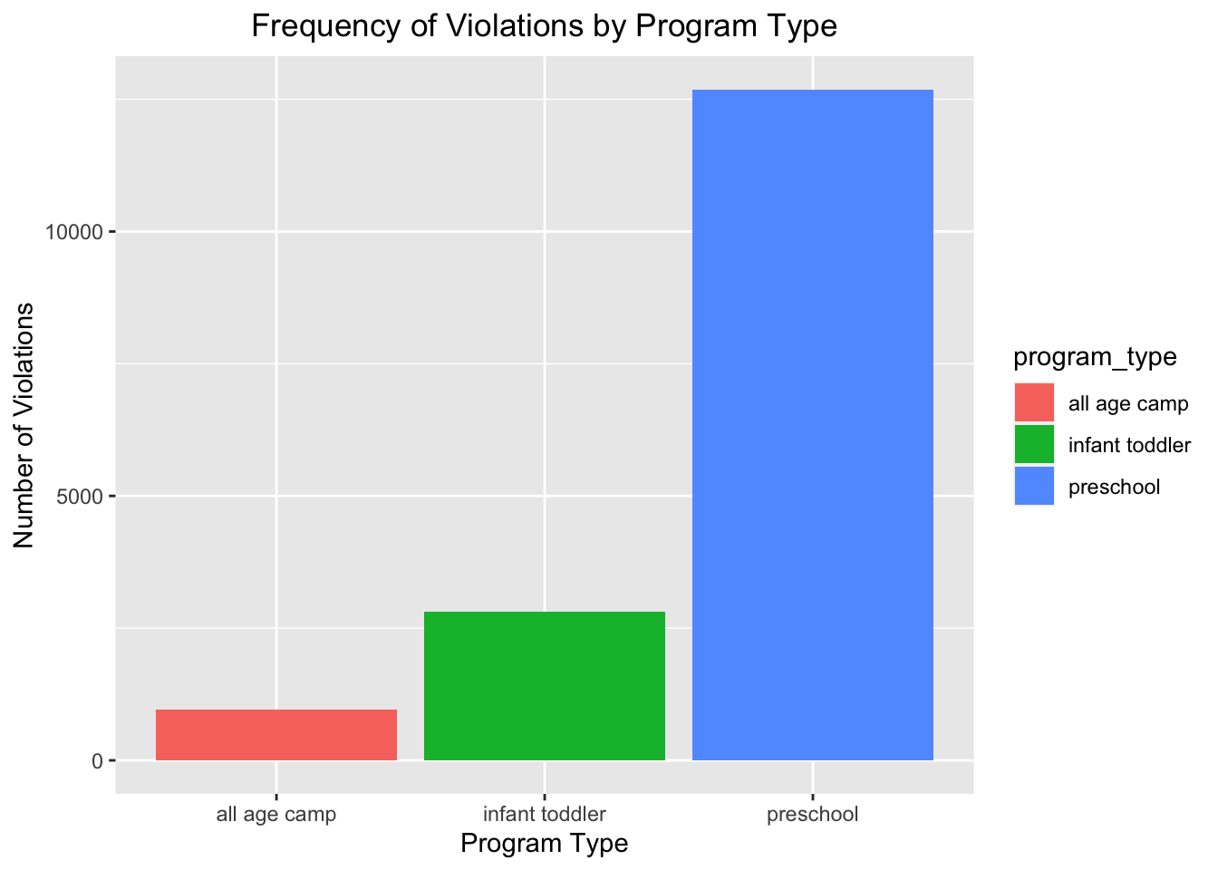

Interpretation

From the histogram plot above, we can learn that preschool has the greatest number of violations.

Number of violations by violation category

Histogram plot

frequency_violation_category = childcare_inspection_df %>% 
  drop_na(violation_category) %>% 
  count(violation_category) %>% 
  mutate(
   violation_category = fct_reorder(violation_category, n)
    ) %>% 
  ggplot(aes(x = violation_category, y = n, fill = violation_category)) + 
  geom_bar(stat = "identity") + 
  labs(
    title = "Frequency of Violations by Violation Category",
    x = "Violation Category",
    y = "Number of Violations",
    fill = "program_type") +
  theme(axis.text.x = element_text(angle = 0, hjust = 0.5),plot.title = element_text(hjust = 0.5))
frequency_violation_category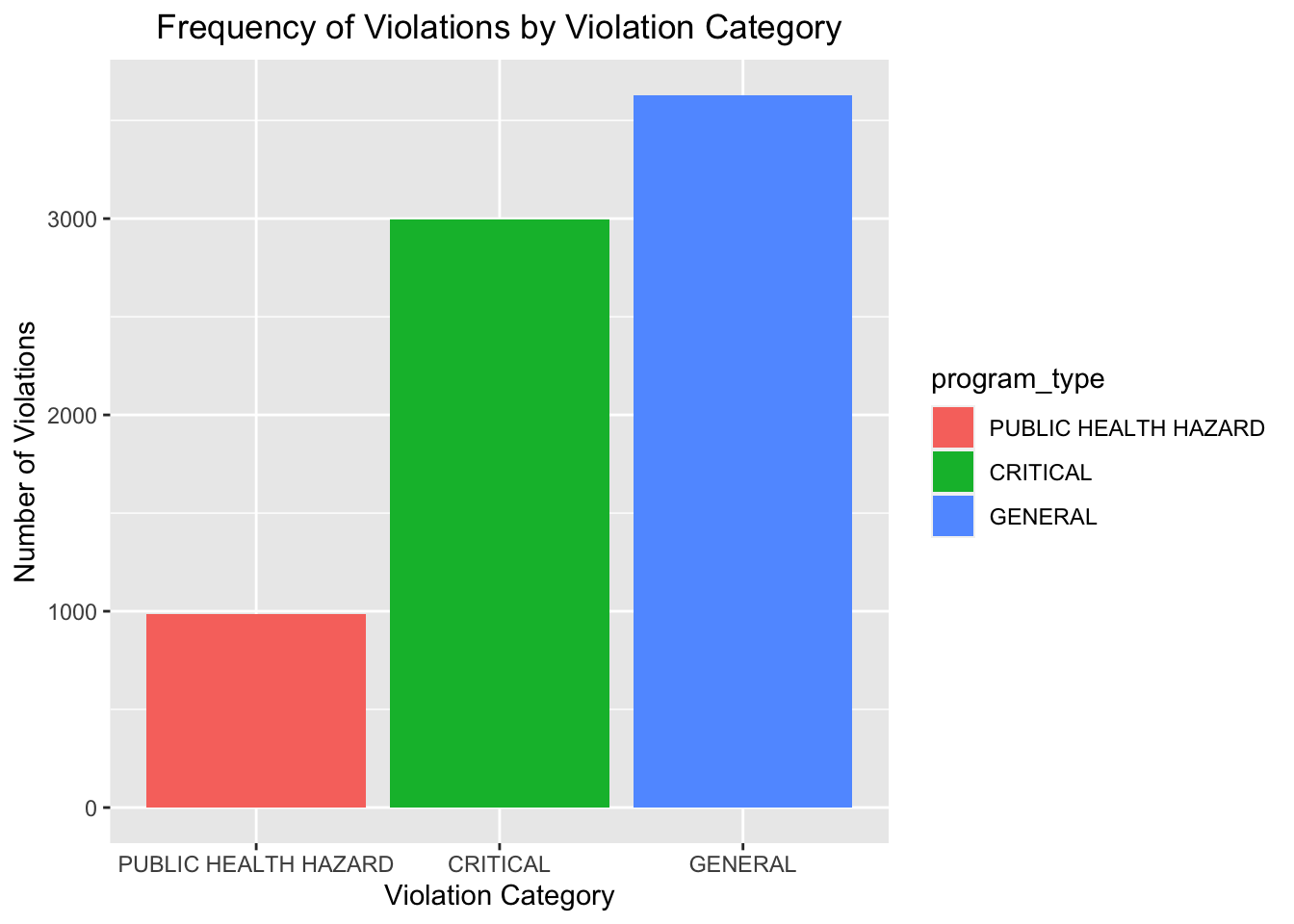 

Interpretation

From the histogram plot above, we can learn that most of the violations belong to general violation category.